shapedRF
Shaped pulses has been widely used to increase excitation bandwidth, achieve desired profile over the entire bandwidth, and improve polarization and coherence transfer efficiencies in numerous NMR experiments. To this end, shapedRF was provided as a general interface for routine patterns (such as Sinc, Gaussian, Rectangle, etc.), external shape files and complex mathematical expressions.
Turn to hardRF for most common used rectangle or hard pulses.
Create a pulse
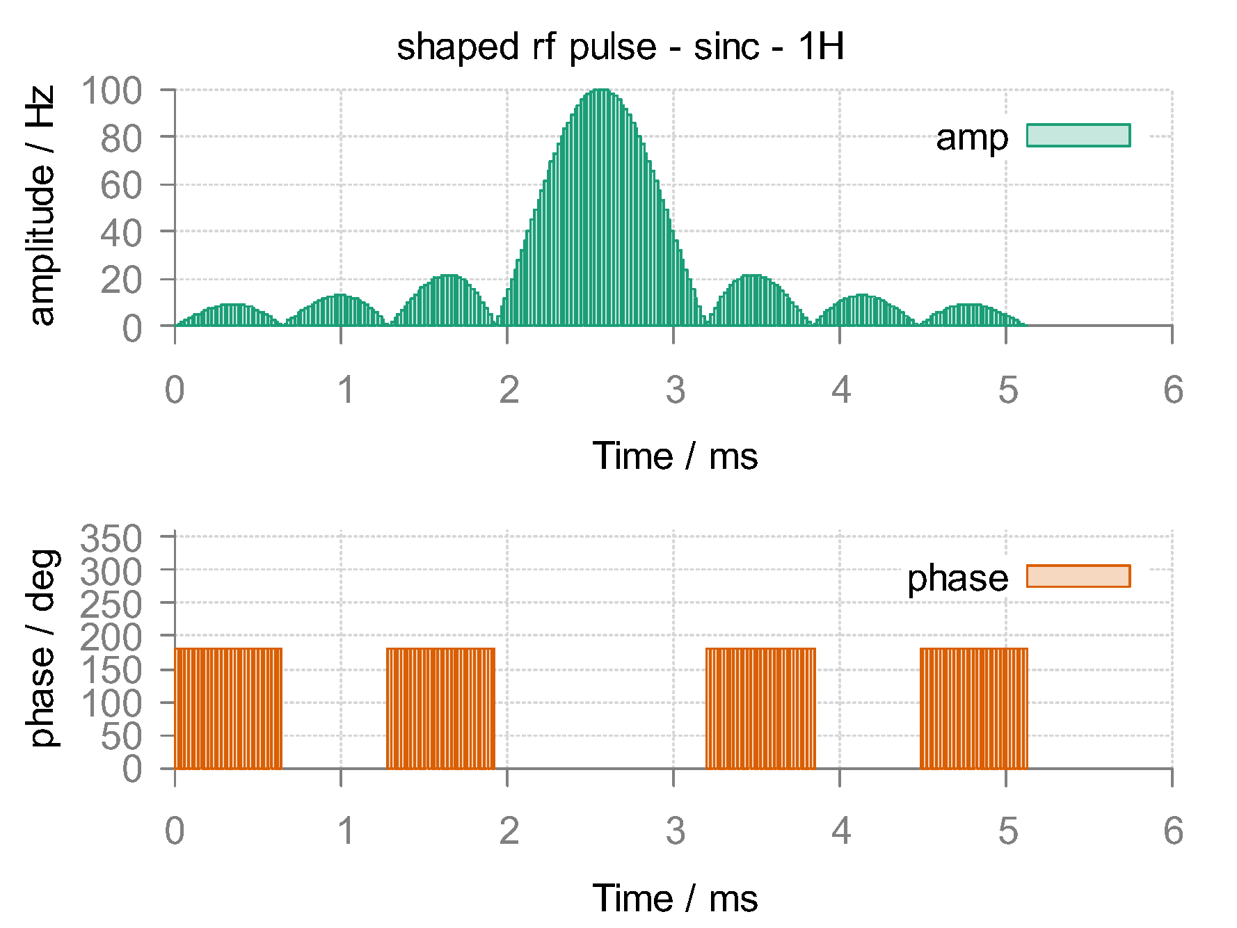
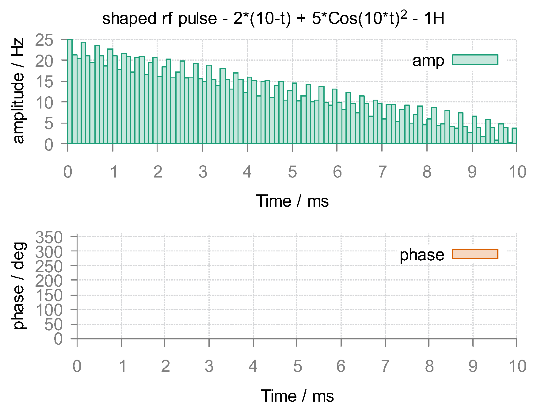
The syntax to create a shaped pulse is simple:
local rf = shapedRF{}The parameter structure is summarized as follow:
Parameter Mandatory/Optional Content width M Pulse duration in ms. pattern M Waveform pattern, described by a string.
(1) Routine patterns. valid types include
"rect","sinc","gauss","hamming","rand","rand_spline". Note that the default maximum amplitude is normalized as 1 Hz.(2) Mathematical expressions. You can define an analytical waveform wih the syntax of computer algebra system YACAS, e.g.
"2*(10-t) + 5*Cos(10*t)^2".(3) External files. External shape can be imported by the file name with suffix
".RF". Click2ms_amp_phase.RFand2ms_ux_uy.RFfor sample files to generate customized pulses in amp/phase (Hz/deg) and ux/uy (Hz/Hz) modes respectively. Note that for the phase range in amplitude-phase mode, both [-180~180] and [0-360] are supported.step O Pulse steps. For pulse shape created by routine patterns or mathematical expressions, step is required. max_amp O Maximum amplitude in Hz, useful for scaling pulse generated with routine patterns. mode O Pulse format, default is "amp/phase". If your external shape is in ux/uy mode,"ux/uy"should be explicitly specified.channel O Nuclear isotope(s) for this pulse, default is "1H". For other nuclei, explicit nuclear isotope such aschannel = "13C"orchannel = "1H|13C"is required. Note for more channels, you only need to seperate the phase for each channel with |.
Pulse operation
Pulse plot
plot(rf)
Mode switch
rf:switch("ux/uy")      -- into ux/uy mode.
rf:switch("amp/phase")  -- into amp/phase mode.
Pulse save
write("raw.RF", rf) -- pulse shape will be stored in customized format of spin-scenario.
Export pulse
rf:export("bruker", "exp.RF") -- pulse shape will be exported as specified ("bruker" and "varian" currently supported).
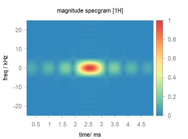
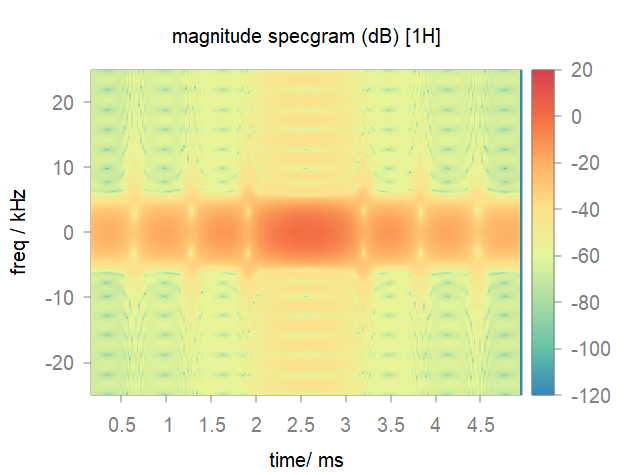
Time-frequency analysis
We provide a STFT based function specgram for the characteristics of shaped pulse.
specgram{}The parameter structure is summarized as follow:
Parameter Mandatory/Optional Content rf M The pulse object.. wlen M Window length. window O Window function in string such as "hammning"(default) ,"gauss", etc.overlap M Overlap ratio. nfft M FFT number. style O Output style of the figure in string. "amp"for the magnitude specgram,"dB"for the magnitude specgram in 20*log and"phase"for the phase specgram.Note
The pulse shape should be in
ux/uymode before the specgram analysis.
Demo script